Lab 12: Poles and Zeros
Introduction
A transfer function serves as a mathematical representation designed to elucidate a linear time-invariant dynamic system. Poles and zeros within a transfer function are crucial concepts facilitating the analysis and manipulation of systems. The system's stability is contingent upon its poles. Stability is achieved when the system is bound to a finite value. Asymptotic stability is realized when the count of real poles is below zero, whereas instability arises if there is at least one pole exceeding zero. Leveraging this understanding, a MATLAB script was developed to experiment with diverse functions and their corresponding impulses.
Procedure
Part 1
The transfer functions corresponding to the system were derived through a differential equation. Initially, the Laplace Transform was employed to transition the equation from the time domain to the complex domain. Subsequently, the poles and zeros of the transfer function were identified and graphed on a pole-zero map. By interpreting the data gleaned from the Pole-Zero map, it becomes possible to ascertain the system's stability status—whether it is stable, asymptotically stable, or unstable—alongside an examination of the impulse response. The initial differential equation is presented in Equation 1.

Upon initially transitioning this equation into the complex domain, the poles and zeros are discerned. Equation 2 provides the transfer function for this system.
𝐻(𝑠) = 1/(𝑠+1)
Equation 2
In this equation, zeros are evident at zero, and poles are located at the negative one. Additionally, the Impulse Function of the equation was examined. Upon observing the graph, it becomes apparent that the function is stable, converging to zero as time approaches infinity. These graphical representations can be viewed in Figures 1 and 2, respectively.

Figure 1: Pole-Zero map, equation 1.
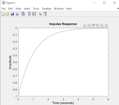
Figure 2: Impulse response graphed, equation 1
After executing these procedures, the second differential equation, as presented in Equation 3, is solved employing identical techniques and steps.

Zeros of this function were identified at 3 and 4, while the poles are characterized by -1, -2+i, and -2-i, as determined through the corresponding transfer function outlined in Equation 4. This system is deemed unstable, demonstrating unbounded growth as time advances toward infinity. The pole-zero map and impulse responses of this equation are presented in Figures 3 and 4, respectively.


Figure 3: Pole-zero map, equation 3.

Figure 4: impulse response graphed, equation 3
Finally, a third differential equation is presented in Equation 5, and the same procedural steps are applied as previously to determine the poles and zeros of the equations. Upon transitioning to the complex domain, the corresponding transfer function is identified as 𝐻(𝑠) = (𝑠−7)(𝑠−3). Zeros of this system are evident at 3 and 7, while the poles are located at 0, -1, -2 + i, and -2 – i. Notably, this system exhibits asymptotic stability, with the poles situated on the left-hand side of the x-axis and converging at approximately 4.25 as time progresses toward infinity. Figures 5 and 6 showcase the PZ-map and Impulse response of this function, respectively.

Equation 5


Figure 5: Pole-zero map, equation 5.

Figure 6: impulse response graphed, equation 5
The subsequent phase in the laboratory experiment involved creating three third-order transfer functions capable of generating stable, asymptotically stable, and unstable impulse responses. These functions are defined in a manner that ensures each function consistently includes a minimum of two zeros. In the case of the stable function, the transfer function employed was:

Equation 6
By examining Equation 6, it becomes evident that the function is stable, given that all poles are situated in the negative region of the x-axis and converge to zero as time approaches infinity. The corresponding Pole-Zero maps and impulse responses for this particular transfer function are displayed in Figures 7 and 8.

Figure 7: pole-zero map, equation 6

Figure 8: impulse response mapped, equation 6.
To describe the asymptotically stable system, consider the transfer function:

Utilizing Equation (7), it is evident that the function is asymptotically stable, given the system's decay approaching zero as time progresses. The corresponding Pole-Zero map and Impulse Response for this transfer function are depicted in Figures 9 and 10, respectively.

Figure 9: Pole-zero map, equation 7

Figure 10: impulse response mapped, equation 7
Concluding with the unstable impulse response, employing the identical steps and processes as before, consider the transfer function:

Equation 8
Utilizing this equation, it becomes evident that the function is unstable, given the presence of one or more poles in the positive region of the x-axis. The corresponding Pole-Zero maps and impulse responses for this transfer function are illustrated:

Figure 11: Pole-zero map, equation 8.

Figure 12: impulse response mapped, equation 8.
The following figures listed above represent the pole-zero maps and impulse responses of their respective equations.
PART II
The subsequent phase of the laboratory involved taking a function representing a circuit with Resistors, Inductors, and Capacitors (RLC circuit) in variable form and transforming it from the time domain to the Complex Domain in a general format. This process yielded the determination of the transfer function, expressed as:

Equation 9
Employing this general form, the values assigned in the laboratory manual for R, L, and C—namely, R=40 Ω, 𝐿 = 3 𝑚𝐻, and 𝐶 = 5 𝜇𝐹—were substituted. With these values, both the impulse response and step response were graphed, as depicted in Figures 13 and 14, respectively. Additionally, the poles and zeros of this function were identified: zeros at 0 and poles at 0 + 70.7i and 0–70.7i. This information indicates the system's stability, as all poles are situated in the negative segment of the x-axis. The Pole-Zero map of this function is illustrated in Fig. 15.
The subsequent step in the script involves maintaining the same function utilized for the RLC circuit while varying the resistance values. Lower resistance results in a reduced amplitude of the impulse response and smaller oscillations. Conversely, a decrease in resistance leads to a significant increase in the magnitude of the poles.

Figure 13: RLC Impulse response

Figure 14: RLC Step response

In this section of the laboratory experiment, a transfer function is provided, and the objective is to ascertain its stability and understand the reasons behind any instability. The given function is:

Equation 10
Zeros were computed at 3 and 4, while poles were identified at -1–i, -1 + i, and 1. Since there is a pole in the positive x-domain, the function is determined to be unstable. Subsequently, pole-zero cancellation is employed to eliminate any redundant zero-pole pairs that do not impact the overall graph. With this cancellation, the function transforms from unstable to asymptotically stable, converging to zero as time approaches infinity. The resulting impulse response curves are depicted.

Figure 16: Impulse response mapped, equation 10
CONCLUSION
In summary, the transfer function proved effective beyond the scope of class lectures. MATLAB facilitated the identification of poles and zeros, aiding in the determination of impulse responses and pole-zero maps.Transfer functions are crucial in signals and systems as they provide a mathematical representation of the relationship between input and output in a system. They help analyze and design systems by simplifying complex interactions. Poles and zeros of a transfer function, depicted in pole/zero maps, offer insights into system stability and behavior. The distribution of poles and zeros influences characteristics such as damping, frequency response, and transient response, making pole/zero analysis vital for understanding and optimizing system performance in fields like control theory and signal processing.


Comments
Post a Comment